Keep the Probability: When Soft Labels Beat Binary Thresholds at Catching Degrading Agents
Keep the probability — don't collapse it to a pass/fail bit. We turned the "soft metrics flagged it" vignette — a self-optimizing agent that games its benchmark while its true quality quietly decays — into a head-to-head detection experiment, scoring every soft metric against its thresholded twin on identical data. A threshold counter placed at the usual τ*=0.50 is blind to degradation that stays above the bar; the soft detector reads the shift in the full quality distribution without needing to know where to put the bar. The soft advantage is real but conditional: biggest (~+0.3 AUROC) exactly where the quality signal is clean, narrowing as observation noise grows. And at a matched false-positive budget, soft flags degrading agents in ~2 epochs to binary's ~10 — catching all of them where binary misses 12%.
We've argued for a while that probabilistic (soft) labels beat binary good/bad classifications for catching agents whose quality is quietly drifting downward. Until now that claim lived in a narrative — a vignette about a self-optimizing agent that keeps passing its benchmark while its real output quality decays. A vignette is not evidence. So we built the experiment.
The setup is a head-to-head: every soft metric is paired with its binary analogue — the same metric computed on the proxy thresholded at τ*=0.50 — and both detectors are scored as real classifiers on identical interaction streams. We report AUROC, AUPRC (critical in imbalanced settings), partial AUROC at low FPR, time-to-detection at fixed FPR, market-level selection signals, and calibration. Same data, same metric definition, the only difference is whether you keep the full probability p or collapse it to a 0/1 at the threshold.
The degrading-agent model
The generative model carries two signals per interaction, and the gap between them is the whole point:
benchmark— the screening signal acceptance is based on. A self-optimizing agent games this: it keeps the benchmark high regardless of falling quality, so its interactions keep getting accepted.p— the true-quality proxy. For a degrading agent this drifts downward, but it stays above the binary threshold. The quality floor sits above τ*=0.50.
That second property is what makes the detection problem interesting. A threshold-counting detector watches interactions keep clearing the bar and sees almost nothing. Only the shift in the full quality distribution — which the soft label preserves and the threshold throws away — reveals the degradation.
We run this in two regimes: a realistic one with heterogeneous agents and an uncertain degradation floor (the headline results below), and an easy baseline with a homogeneous population (which we use to expose a measurement artifact at the end). Both sweep multiple adversarial base rates and seeds, with degradation trajectories (linear / exponential / step / sigmoid) and onset times varied across agents.
Result 1: Soft beats binary — but only where the signal is clean
The honest test is a regime where detection is a genuine statistical problem: benign agents that vary in quality (so their lower tail overlaps mildly-degraded ones) and a per-agent, uncertain degradation floor (so some agents barely degrade). There the per-agent toxicity detector produces a real response surface — not a wall of perfect scores. Here is AUROC across observation noise (proxy_noise) and per-epoch quality jitter, for soft, binary, and their difference:
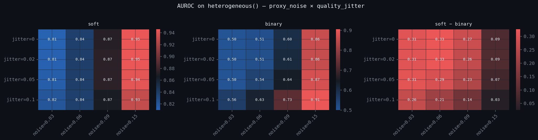
Soft AUROC lands in a genuine 0.81–0.95; binary ranges from 0.50 (blind) to 0.91. Sweeping observation noise at fixed quality_jitter = 0 (the top row of the heatmap):
| proxy_noise | soft AUROC | binary AUROC | gap |
|---|---|---|---|
| 0.03 | 0.810 | 0.500 | +0.310 |
| 0.06 | 0.837 | 0.510 | +0.327 |
| 0.09 | 0.872 | 0.599 | +0.273 |
| 0.15 | 0.946 | 0.860 | +0.086 |
Three things stand out:
- The soft advantage is real but conditional. It's largest (~+0.31 AUROC) exactly in the clean-signal regime — low observation noise — which is the operating point a mature monitoring system aims for, and where binary is near-blind (AUROC 0.50, AUPRC ≈ base rate). As observation noise rises, binary "catches up" (enough quality mass finally crosses τ*=0.50) and the gap shrinks to +0.03–0.09. Keep the probability matters most precisely where your signal is good.
proxy_noiseis the dominant axis. Both detectors improve left-to-right; the soft–binary gap is governed mostly by how much observation noise blurs the threshold.- A subtle interaction the easy regime can't show: per-epoch quality jitter helps the binary detector (rightmost panel, lower rows) — it widens the distribution so more degrading interactions dip below the threshold — while being roughly neutral for soft.
Reproduce the full proxy_noise × quality_jitter grid with one flag:
(The naive run on the default generator pins soft at a perfect AUROC 1.00 — that's a ceiling of the model, not a result. We unpack why at the end.)
Result 2: Time-to-detection — 2 epochs vs 10
The more operationally useful question isn't "can you eventually tell them apart" but "how fast." We calibrate each detector to a fixed false-positive rate (FPR ≤ 0.05) on benign agents, then measure epochs-from-onset until it flags a degrading one.
| variant | median epochs from onset | detection rate |
|---|---|---|
| binary | 9.93 | 0.88 |
| soft | 2.13 | 1.00 |
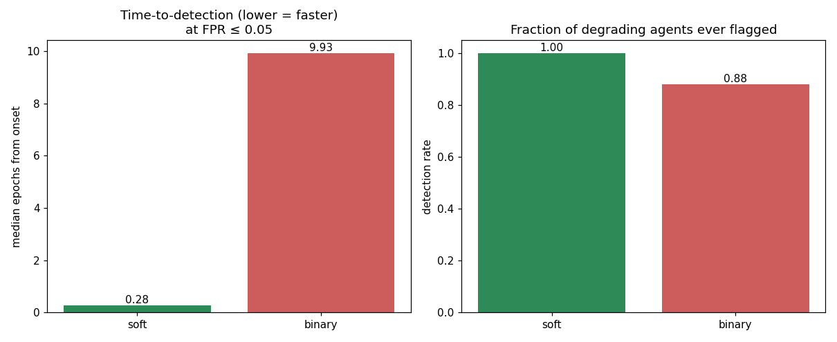
At the same false-positive budget, the soft detector flags degradation in about 2 epochs and catches 100% of degrading agents. The binary detector takes nearly 10 epochs and misses 12% of them entirely — those are the agents whose gamed benchmark keeps them above the threshold long enough that the trailing-window count never crosses the alarm line.
A note on rigor: an earlier version of this measurement scanned for detections over a wider epoch window than the one the FPR threshold was calibrated on, which let pre-onset windows artificially deflate the soft TTD (we'd reported 0.28 epochs). After aligning the scan and calibration windows — flagged in review on the PR — the honest figure is 2.13 epochs. Still a ~5× speedup, just not a magic one.
Result 3: Market-level adverse selection
Toxicity and uncertain_fraction are per-agent detectors. Quality-gap, conditional-loss, and spread are selection metrics — they compare accepted vs rejected interactions across a quality mixture, so they're only well-posed at the market level. The runner now reports all of them automatically.
The soft versions read a real adverse-selection signal; the binary versions flatten to noise:
| metric | variant | br=0.05 | br=0.10 | br=0.20 | br=0.35 | br=0.50 |
|---|---|---|---|---|---|---|
| quality_gap | soft | −0.106 | −0.100 | −0.085 | −0.066 | −0.048 |
| quality_gap | binary | 0.000 | 0.001 | 0.001 | 0.004 | 0.003 |
| conditional_loss | soft | −0.021 | −0.019 | −0.015 | −0.011 | −0.007 |
| conditional_loss | binary | 0.000 | 0.000 | 0.000 | 0.001 | 0.000 |
| spread | soft | −0.043 | ... | −0.031 | ... | −0.015 |
| spread | binary | −0.001 | ... | −0.000 | ... | 0.000 |
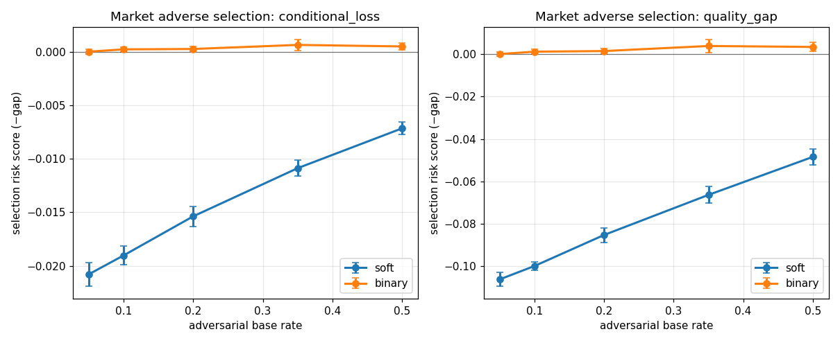
The soft quality-gap and spread are consistently negative (the signature of adverse selection), strongest in the rare-adversary regime. Their binary twins read ~0.00 everywhere: once you threshold, accepted and rejected look identical because the gamed agents all sit on the "accept" side of the line. The detection framework now automatically includes spread alongside the original two selection metrics.
Result 4: Calibration
Finally, how much predictive resolution does thresholding actually destroy? We score the soft probability p against ground-truth outcomes versus its hard-thresholded twin 1{p ≥ τ\*}:
| Brier | ECE | |
|---|---|---|
| soft | 0.151 | 0.054 |
| binary | 0.183 | 0.183 |
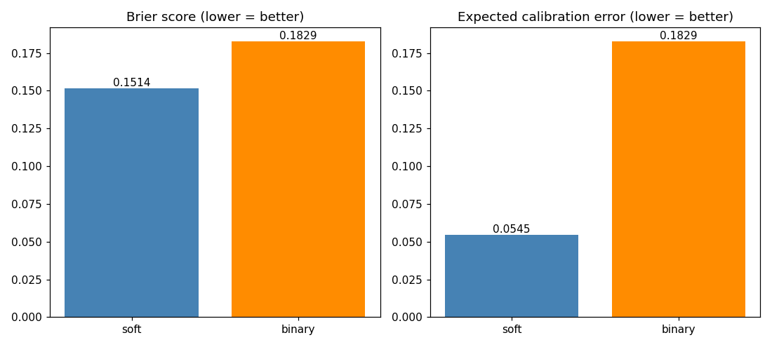
The binary prediction's expected calibration error equals its Brier-style miss because a 0/1 prediction is maximally overconfident — it claims certainty it doesn't have. The soft probability stays well-calibrated (ECE 0.054).
A note on the easy regime: why the naive numbers say "AUROC 1.00"
Run the same experiment on the default (homogeneous) generator — every benign agent pinned to one quality, a fixed degradation floor — and the soft toxicity detector scores a perfect AUROC = 1.000 at every base rate, with binary trailing at ~0.91–0.96:
| base rate | soft AUROC | binary AUROC |
|---|---|---|
| 0.05 | 1.000 ± 0.000 | 0.925 ± 0.115 |
| 0.10 | 1.000 ± 0.000 | 0.950 ± 0.061 |
| 0.20 | 1.000 ± 0.000 | 0.912 ± 0.064 |
| 0.35 | 1.000 ± 0.000 | 0.964 ± 0.036 |
| 0.50 | 1.000 ± 0.000 | 0.945 ± 0.040 |
We deliberately don't lead with this. Those 1.000s are a ceiling of the generator, not a measure of detection power: with benign agents pinned to a single quality and ~50–100 interactions averaged per agent, the two classes are separated by ~7.8 standard deviations (d′ ≈ 7.8) and never overlap, so AUROC ≈ 1.0 is a near-mathematical certainty. The same ceiling shows up in AUPRC — at a 5% base rate soft sits at 1.000 while binary collapses toward ~0.37, directionally real (thresholding hurts most when positives are rare) but with a saturated soft endpoint. What survives de-saturation is the direction and mechanism (a threshold detector's benign score is literally 0.000 because nothing crosses τ*=0.50) and the noise-dependence in Result 1 — not the absolute 1.00. Stress tests and what a genuine power test requires: docs/notes/detection_soft_ceiling_caveat.md.
Why this matters
The takeaway isn't that soft labels are better in the abstract. It's that the specific failure mode of modern self-optimizing agents — gaming the acceptance signal while real quality decays — is invisible to a threshold-counting detector at the natural τ*=0.50, and visible to a distributional one. (How much of that is the threshold placement vs the soft signal itself, we pin down in Limitations below — the honest answer is: more placement than we first thought.)
And it's conditional in a way that favors good monitoring: the soft edge is largest exactly where the quality signal is clean and low-noise — the regime a mature system works to reach — and narrows only as observation noise washes the threshold out. If your safety monitoring collapses a calibrated probability to a pass/fail bit, you are throwing away exactly the signal that catches the agents you most want to catch, in the regime where you could most easily have caught them — and you find out ~5× slower when you do.
Limitations: what follow-up ablations revised
We ran four ablations to pressure-test the "soft beats binary" claim. They narrowed it substantially — and we'd rather say so than ship the tidy version.
1. Most of binary's "blindness" was a mis-placed threshold, not lost information. The binary detector thresholds at τ*=0.50, but the class boundary sits up at ≈0.74–0.85 (degrading floor → benign quality). Sweeping the threshold, the binary detector matches soft at clean signal and beats it at higher noise once τ* is placed near the boundary (best τ* ≈ 0.60–0.80). A threshold calibrated on benign agents alone lands in roughly the right place — no degradation labels needed. So thresholding doesn't "discard the distributional signal" — putting the threshold at 0.50 does. (note)
2. Under proxy drift, a once-calibrated alarm fails silently — and for soft and binary alike. If the proxy's calibration drifts (the monitor gradually over-reports quality), a threshold calibrated once sees its detection rate collapse from ~0.46 to ~0.00, while AUROC stays at 0.88–0.91 the whole time. A monitor can look perfect on AUROC and catch nothing in production. This hits soft and binary equally; neither escapes recalibration. The operational lesson — track realized false-alarm/detection rates at your committed threshold, don't trust AUROC alone — matters more than soft-vs-binary. (note)
3. Soft's genuine, narrower edge: rank-invariance to recalibration. Where soft does cleanly win is scale drift — when the proxy loses resolution (its range compresses), soft's AUROC is unchanged (the per-agent mean is an affine, order-preserving transform) while a fixed-threshold binary detector collapses to chance, because the threshold no longer sits inside the data. Soft needs no threshold to go stale. That's a real advantage — but it's about recalibration-free ranking, not superior raw detection power.
4. Against an adaptive adversary, soft is genuinely harder to fool. When an agent that games its benchmark gets to choose how to evade, lowering its mean quality is caught by soft and by a boundary-placed threshold alike. But a threshold counts crossings, which depend on the distribution's shape as well as its mean — so an adversary can hold real quality degraded (mean ≈0.81) while tightening its output to sit just above τ*, producing almost no crossings: it slips past even the well-placed binary detector (catch rate 1.00 → 0.18) while soft still catches it (1.00). The mean has only one way to look benign — by being benign on average — so the only way to evade soft is to actually raise quality. (note)
Net: with a boundary-placed, regularly-recalibrated threshold, a binary detector is competitive on static discrimination; soft's durable advantages are convenience (no τ* to tune), rank-robustness to proxy recalibration, and resistance to adversarial distribution-shaping. The headline above holds at the naive operating point most systems actually use — but it is not the structural impossibility the phrase "by construction" suggests.
Everything here is reproducible:
PYTHONPATH=. python experiments/run_detection_experiment.py          # 5 base rates × 10 seeds
PYTHONPATH=. python experiments/run_detection_experiment.py --smoke  # quick
The runner now automatically produces tables for:
- AUROC by base rate
- AUPRC (Area Under the Precision-Recall Curve)
- Partial AUROC at low FPR (FPR ≤ 0.05 and 0.01)
- Time-to-detection at calibrated FPR
- Market adverse selection (including spread)
- Calibration
The full detection module (swarm/detection/), matched detectors (toxicity + uncertain_fraction per-agent; quality_gap + conditional_loss + spread at market level), generative model, and tests landed in PR #450. Subsequent improvements (pAUROC + proper AUPRC surfacing, plus the spread and uncertain_fraction matched detectors and a 2D sensitivity-grid runner) landed in PR #453.
Disclaimer: This post uses financial market concepts as analogies for AI safety research. Nothing here constitutes financial advice, investment recommendations, or endorsement of any trading strategy.