τ* ablation: most of binary's "blindness" is threshold placement, not lost information

Date: 2026-05-25 Follows: detection_informative_regime.md, detection_2d_grid_heterogeneous.md. Bottom line: The headline "thresholding is structurally blind to degradation" is substantially overstated. Binary's failure at τ=0.50 is mostly because 0.50 is the wrong threshold — it sits far below the class boundary. With the threshold tuned to the boundary, the binary detector matches soft at clean signal and beats it at higher noise. Soft's genuine, narrower advantage is that it is threshold-free*.

Setup

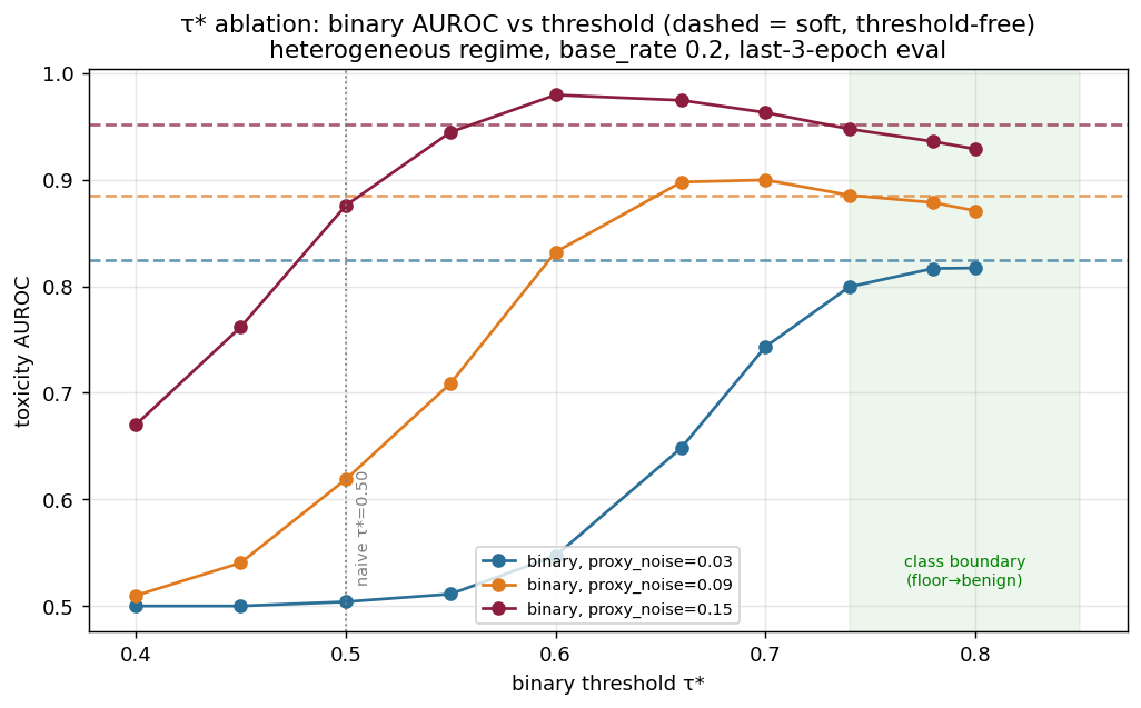
The soft toxicity detector reads the full proxy p (no threshold). Its binary twin scores the fraction of accepted interactions with p < τ*. We sweep τ* on the heterogeneous regime (StreamConfig.heterogeneous(): benign quality ≈0.85, degrading floor ≈0.74, both with per-agent spread), base rate 0.2, last-3-epoch eval, 8 seeds × 160 agents, at three observation-noise levels.

The default τ=0.50 used everywhere else in this work sits far below* the actual class boundary (degrading floor 0.74, benign 0.85). That is the crux.

Binary AUROC vs τ*

proxy_noise	soft	τ=0.40	0.45	0.50	0.55	0.60	0.66	0.70	0.74	0.78	0.80
0.03	0.825	0.500	0.500	0.504	0.511	0.547	0.648	0.743	0.799	0.817	0.817
0.09	0.885	0.510	0.541	0.619	0.709	0.832	0.898	0.900	0.885	0.878	0.871
0.15	0.952	0.670	0.762	0.876	0.945	0.979	0.974	0.963	0.948	0.936	0.929

Soft vs binary@0.50 vs binary@best-τ*

proxy_noise	soft	binary @ 0.50	binary @ best-τ*	best τ*	residual (soft − best)
0.03	0.825	0.504 (blind)	0.817	0.80	+0.008
0.09	0.885	0.619	0.900	0.70	−0.015
0.15	0.952	0.876	0.979	0.60	−0.027

What this means

1. τ*=0.50 is simply mis-placed. The discriminative region is the gap between the degrading floor (≈0.74) and benign quality (≈0.85). A threshold at 0.50 puts almost no probability mass on either side for either class, so the binary detector sees nothing — AUROC ≈ 0.50 at clean noise. That is a threshold-choice failure, not evidence that the hard label discards the signal.

2. Tuned to the boundary, binary matches or beats soft. The optimal τ tracks the boundary and shifts down as noise grows (0.80 → 0.70 → 0.60). At its optimum the binary detector ties soft in the clean regime (+0.008) and exceeds it at moderate/high noise (−0.015, −0.027). A single well-chosen threshold can be a better* feature than the mean 1−p, because it concentrates on the crossing region instead of being pulled around by both tails.

3. So the real soft advantage is being threshold-free — not superior discrimination. Soft needs no τ. Binary needs the threshold placed near a boundary that is (a) unknown a priori, (b) different per agent (the floor varies), and (c) drifting as agents degrade. A fixed τ goes stale; the threshold-free detector does not. That is a genuine operational benefit, but a much narrower claim than "thresholding is structurally blind."

Honest caveats on this ablation

• The best-τ* column is an oracle (threshold picked with labels in hand), so it is an optimistic upper bound for binary. The fair question is whether you could place τ that well without* labels. You largely can: a benign-FPR-calibrated threshold lands in the benign lower tail (~0.70–0.80), which is exactly where the optimum sits — so the "0.50 is just mis-placed" conclusion survives even under label-free calibration.
• Soft is still automatically well-placed and drift-robust, which is why we keep it as the default; this ablation narrows why it helps, it doesn't reverse the recommendation.

Implication for the blog post

docs/blog/soft-vs-binary-detection.md currently frames binary as "structurally blind … thresholding discards precisely the distributional signal." That is true at τ=0.50 but misleading as a general statement. The post should be updated to: (a) note that 0.50 is below the class boundary, and (b) reframe soft's advantage as threshold-free / drift-robust rather than strictly more discriminative*. Flagged as a follow-up.

Reproduce

import numpy as np
from swarm.detection.degradation import StreamConfig, PopulationConfig, generate_population
from swarm.detection.detectors import MatchedDetectors
from swarm.detection.curves import compute_curve, per_agent_scores

soft = MatchedDetectors()
for pn in (0.03, 0.09, 0.15):
    cfg = StreamConfig.heterogeneous(proxy_noise=pn); n = cfg.n_epochs; es, ee = n - 3, n
    streams = generate_population(PopulationConfig(n_agents=160, base_rate=0.2, stream=cfg), seed=0)
    s, lab = per_agent_scores(streams, soft.soft_toxicity, es, ee)
    print(pn, "soft", round(compute_curve(s, lab).auroc, 3))
    for t in (0.50, 0.60, 0.70, 0.80):
        b = MatchedDetectors(tau_star=t)
        s, lab = per_agent_scores(streams, b.binary_toxicity, es, ee)
        print("   τ*", t, round(compute_curve(s, lab).auroc, 3))